It is easy to see the merit in a Stock Rank based on high Quality and high ( i.e. cheap) Value. And yet, over the last year or so, it is the expensive but high quality stocks which have performed well: the so-called "high flyers". But even while acknowledging that this is true for now, we can realise that there must come a point where a stock is too expensive, no matter how good it is.
Conversely, if a stock is very cheap then there may be a good reason for that. Perhaps the market is sufficiently unimpressed that even at a knock-down price there are enough doubts to prevent it being snapped up.
It seems equally simplistic to choose stocks with high Q and high V (both good and cheap - but why are such bargains lying around?) or alternatively to choose high Q and low V (can it be right to be deliberately attracted to already expensive stocks, even if they are high quality?)
The Stock Rank provides one approach: by combining Q V and M it effectively gives the QM side a bit more influence than the V side while ensuring there is a V component to avoid chasing momentum to increasingly crazy heights. It definitely works. Last year (2017) the NAPS portfolio not only had superb performance but quite extraordinarily low volatility as well. I am still slightly astonished by how it managed the low volatility that it did.
I wanted to have a more rigorous understanding of how Q and V were interacting, so I though I would have a quick look at the contingency table for Q versus V. For the purposes of this post, it is enough to know that this is a very simple application of Bayes Theorem. We start with a "prior" which is the median yearly return for all stocks in the sets we are considering. We then look at how the values of the Q and V rank will change the probability of achieving at least this median return. These are reported as a likelihood ratio, where values over 1 indicate a higher probability and values under 1 indicate a lower probability. Because we are taking (Q,V) as a pair which vary together and have interdependence (rather than two separate independent variables) we get a "contingency table". [Right-click 'view image' for a bigger version as…


v.v.v. interesting
to answer phil h's question
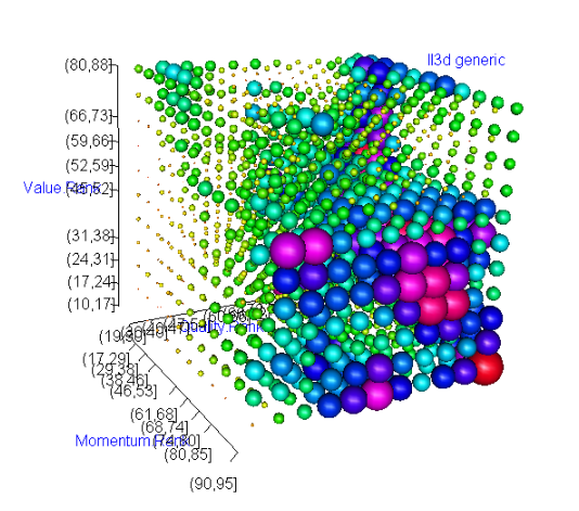
I think it means that if you choose Q > 80 (on the horizontal axis, pick the last two vertical columns), chances are you beat the median return no matter the value rank (vertical axis).
However, if you pick V between 40 and 60 and Q > ~70, your chances are maximised (blue/pink/red bits).
My question is
- what time period (from / to)
- sample size
- what date were the Q and V values taken?
- was this the start of the period (in which case how, cant believe you downloaded X hundred historic reports and transcribed them -or if you did or found a better way, much respect)
- was this the end of the period in which case I am not sure what it is telling me